Hyporthsis

8/30/2013

Roll No : EPGP-04B-103 | Saurabh Prasad |

Indian Institute of Management Kozhikode | Six Sigma : Assignment No 2 |

α= 0.05 and on assumption of equal variances.

X1 bar = 92.3375 & X2 bar = 92.6125

D1 = 2.68 and D2 = 3.13

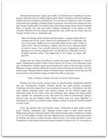
8 step hypothesis procedure:

1. The parameters of interests U1 & U2. We want to know if U1 – U2=0

2. Hypothesis A , µ1 –µ2 = 0 or µ1 = µ2

3. Hypothesis B, µ1 is not equal to µ2

4. The test Static is

5. t 0 = X1 – X2 – 0 / s p √(1/n1 + 1/n2) ( X1 & X2 are Mean )

6. Reject Hypothesis A, if t 0 is greater than t 0.025,14 = 2.145 or if t 0 is lesser than – t 0.025,14 = - 2.145.

7.

D1 & D2 are Standard Deviations

N1 & N2 are the count or sample readings

S p Square is Variance

S p is Square root of Variance

And

8. Conclusion: since – 2.145 is lesser than t 0 = -0.2037 which is lesser than 2.145, the null hypothesis can’t be rejected. Which means that at 0.05 levels , we do not have strong evidence to conclude that catalyst 2 results in a mean yield that differs from the mean yield when catalyst 1 is used.

Q 2

Regression Analysis: Delivery Time versus No of Cases

Weighted analysis using weights in Delivery Time

The regression equation is

Delivery Time = 24.4 + 0.144 No of Cases

Predictor Coef SE Coef T P VIF

Constant 24.439 1.296 18.85 0.000

No of Cases 0.144369 0.006279 22.99 0.000 1.000

S = 15.8430 R-Sq = 96.7% R-Sq(adj) = 96.5%

PRESS = 5486.95 R-Sq(pred) = 96.00%

Analysis of Variance

Source DF SS MS F P

Regression 1 132674 132674 528.58 0.000

Residual Error 18 4518 251

Total 19 137192

Unusual Observations

No of Delivery

Obs Cases Time Fit SE Fit Residual St Resid

17 267 58.20 62.98 0.70 -4.78 -2.45R

R denotes an observation with a large...